
In this article we will discuss how to evaluate X-ray images of welds with a few lines of Python code. For this purpose, the contrast is adjusted during processing, the colors of the image are inverted and possible imperfections are highlighted. The skimage library was mainly used. This library provides classical algorithms and filters for image processing.
Requirements
A Jupyter notebook with Python 3.7 was used for programming. Especially useful is the decoupling from the host system or the use of docker containers. However, this is not absolutely necessary. In order to carry out later, if necessary, deeper analyses with Machine Learning, a TensorFlow Docker Image has been used here. If you do not want to use Docker or just want to see the Python code, you can simply skip the next sections.
Setting up the Docker Image
If Docker is installed, the Jupyter Notebook can be initialized as follows. First download the TensorFlow image (docker pull) and then start it (docker run). Then you can program comfortably via the browser, because the localhost port 8888 is routed to the Web IDE of the container (-p 8888:8888). The option -name tf gives the container the name tf (as an abbreviation for TensorFlow) to be able to call it later more easily. In order to save the created code, a folder “tf” has to be created (mkdir) as well, which is mounted as volume (with the option -v ) in the Docker Container. This folder can also be named arbitrarily, but the paths must be adjusted accordingly.
The following commands must be executed for this:
cd
mkdir tf
docker pull tensorflow/tensorflow:latest-py3-jupyter
docker run -p 8888:8888 --name tf -v /tf:/tf/Entwicklung tensorflow/tensorflow:latest-py3-jupyter
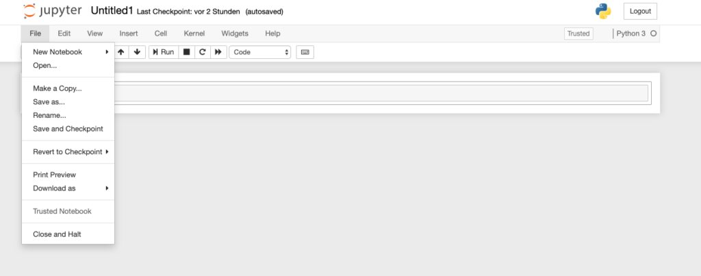
Now a Jupyter Notebook Server is hosted on the local machine. If you follow the instructions in the console, you can then go to the corresponding path http://127.0.0.1:8888/?token=<token> in the browser and create a notebook in the folder ‘Development’. To do this, click on the ‘New’ button in the upper right corner and then ‘Notebook: Python 3‘.
After that you should save the notebook via ‘File’ – ‘Save And Checkpoint’, where ‘Untitled.ipynb‘ is created by a file, which is now also on the host system and thus secured.
Setting up the Python environment
Now the required Python packages must be installed. To do this, you should either work in the Docker Container or with Virtual Environments (if Docker was not used). With the command (docker exec) you can access the console in the container and install the packages via pip. The package scikit-image or skimage will be used for processing and matplotlib for display. Additionally numpy is used for help. For installation the following commands must be executed.
docker exec -it tf /bin/bash
#Console of container
pip install matplotlib numpy scipy scikit-image
The Python script
The first thing to do is to import the different packages. We create a new section in the notebook or our script and insert the following lines:
import numpy as np
import matplotlib.pyplot as plt
import base64
from skimage import feature, io, filters, util, exposure, restoration
from matplotlib.colors import ListedColormap
Then a function is created that adjusts the colors for marking the imperfections and weld defects. This is because different layers of the image are to be superimposed. Therefore the unmarked parts of the layer must be transparent.
def createTransparentMap(cmap):
  # Get the colormap colors
  my_cmap = cmap(np.arange(cmap.N))
  # Set alpha
  my_cmap[:,-1] = np.linspace(0, 1, cmap.N)
  # Create new colormap
  return ListedColormap(my_cmap)
Then a function is defined which can read images base64 encoded. First the formatting of the image string is checked and then a pixel matrix is output. A file could also be loaded using the io.imread method of skimage. However, this file would then have to be mounted. The base64 variant was chosen for use within a possible web service, as this is often used as the standard for RESTful interfaces.
def decode(base64_string):
  # check format
  if isinstance(base64_string, bytes):
    base64_string = base64_string.decode("utf-8")
  # decode
  imgdata = base64.b64decode(base64_string)
  img = io.imread(imgdata, as_gray=True, plugin='imageio')
  # pixel matrix
  return img
To continue, some constants are defined in the script afterwards. A sigma value that is used for edge detection with a canny filter. Two custom color palettes to mark the imperfections and a censure detector to detect features in the image. The weld defects are then automatically detected and marked as a feature of the image.
sigma = 0.6
redMap = createTransparentMap(plt.cm.cool)
blueMap = createTransparentMap(plt.cm.GnBu)
detector = feature.CENSURE()
The actual analysis function for the marking can then be created. For this purpose, the image is first transferred into a pixel matrix with the help of the previously created decode method. Then a sigmoid function is applied to adjust the contrast of the image. In image processing, the sigmoid function is very often used as a standard besides the ReLU. The adjusted matrix serves as input to the Censure detector.
def process_image(baseImage):

  im = decode(baseImage)
  # Correction of image (contrast, noise etc)
  sigmoid_im = exposure.adjust_sigmoid(im)

  #Feature detection
  detector.detect(sigmoid_im)
Afterwards the results of the edge detection are stored in the variables edges1 and edges2. A canny algorithm (with the previously defined sigma) and a Sobel filter are used for this. However, these are not applied to the sigmoid-adapted matrix, because it causes too much noise in the test pattern.
# Compute the Canny filter for two values of sigma
  edges1 = feature.canny(im, sigma=sigma)
  edges2 = filters.sobel(im)
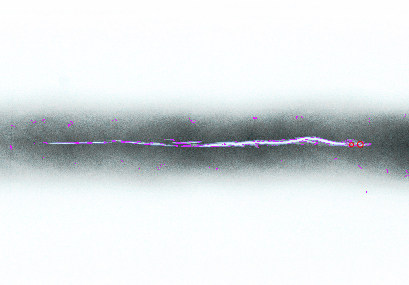
Now that the features and edges of the image have been recognized, they can be displayed with matplotlib. For this purpose, a 1-axis graphic is created and the image planes are drawn with the ax.imshow calls. In the lowest layer the colors of the sigmoid matrix are inverted (util.invert) and then the edges (Canny and Sobel) are drawn with the previously adjusted colors. Afterwards, the detected features of the Censure detector are drawn in with a scatter plot and the graphic is finally presented with plt.show.
# display edges
  fig, (ax) = plt.subplots(nrows=1, ncols=1, figsize=(32, 12), sharex=True, sharey=True)

  #draw pixels
  ax.imshow(util.invert(sigmoid_im), cmap=plt.cm.gray)
  ax.imshow(edges1, cmap=redMap)
  ax.imshow(edges2, cmap=redMap)

  # display censure features
  ax.scatter(detector.keypoints[:, 1], detector.keypoints[:, 0], 2 ** detector.scales, facecolors='none', edgecolors='r')
  ax.axis('off')
  plt.show()
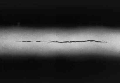
If you now use the function process_image with an example image, this can look like this. A JPEG file was encoded using this tool (in binary format). It represents a typical digital RT image of a weld seam.
sampleImage = '...'
processImage(sampleImage)
Conclusion
This short script shows how an image of a weld seam can be adjusted using simple functions of the skimage library. The parameters and filter functions here have been chosen to detect errors and imperfections on the test image. For practical use, however, it is recommended that these parameters are not rigidly defined, but are selected adaptively. The next steps for embedding the algorithm in a cloud service could be, for example, AWS Lambda or an own React frontend. In addition, the environment with TensorFlow can be used to apply further algorithms e.g. with Machine Learning. To make first steps in image processing, skimage still offers enough filters and options.
sentin EXPLORER
In order to save time and nerves during testing and evaluation, you should use the right tool. The sentin EXPLORER facilitates the evaluation by automatically analyzing and marking of discrepancies.
External and internal characteristics play a role in the evaluation of welds. Non-destructive material testing such as visual inspection (visual inspection – VT) or imaging methods (e.g. radiographic testing with X-rays or gamma rays – RT, or ultrasound with phased array – UT) can be used to examine them for cracks or pores, for example.
More about this in our article:
Do you have questions or comments? Feel free to contact us.